Firms and Market Structures

Firms and Market Structures

What You'll Learn

Every business operates inside a market, and the rules of that market determine how much power the business has over its own prices. A neighborhood coffee shop competes very differently from a regional electric utility. This reading explains why some markets are brutally competitive while others border on monopoly, and how firms in each setting decide whether to keep the lights on or shut the doors.

• How to classify markets using five key characteristics
• The difference between perfect competition, monopolistic competition, oligopoly, and monopoly
• When a firm should shut down versus keep operating
• Short-run and long-run breakeven and shutdown rules
• Economies and diseconomies of scale along the LRATC curve
• Five oligopoly pricing models and how they differ
• How to find a Nash equilibrium from a payoff matrix
• Measuring market concentration with the N-firm ratio and the Herfindahl-Hirschman Index (HHI)

---

The Spectrum of Market Structures

Think of market competition like a dimmer switch, not an on-off toggle. Perfect competition is the brightest setting (maximum rivalry). Monopoly is the dimmest (zero rivalry). Monopolistic competition and oligopoly sit in between.

Five factors tell you where a market sits on this spectrum:

1. Number of firms and their relative sizes
2. Product differentiation: identical or unique?
3. Pricing power: can a single firm move the price?
4. Barriers to entry: how hard is it for newcomers?
5. Non-price competition: advertising, branding, quality

Every market structure is just a different combination of these five factors. The table below gives you the full picture at a glance.

Feature	Perfect Competition	Monopolistic Comp.	Oligopoly	Monopoly
Firms	Many, small	Many	Few	One
Products	Identical	Differentiated	Similar or different	Unique, no close subs
Pricing power	None (price-taker)	Some	Some to significant	Significant
Barriers to entry	Very low	Low	High	Very high
Non-price competition	None	Heavy (ads, branding)	Heavy	Advertising vs. substitutes
Demand curve	Horizontal	Downward-sloping, elastic	Downward-sloping	Downward-sloping, steep
LR economic profit	Zero	Zero	Possible but trends to zero	Possible

---

Perfect Competition

Under perfect competition, many small firms sell identical products. No single firm is big enough to influence the market price, so every firm is a price-taker. It simply accepts the going price and decides how much to produce.

Think of a wheat farmer in a large agricultural market. The farmer checks today's price and ships whatever quantity maximizes profit. If the farmer tried to charge one cent above the market price, buyers would just go to the next farm.

Key Features

• Products are homogeneous (no branding, no quality differences).
• Barriers to entry are very low. New farms can start up easily.
• The firm's demand curve is horizontal at the market price. It can sell as much as it wants at that price.
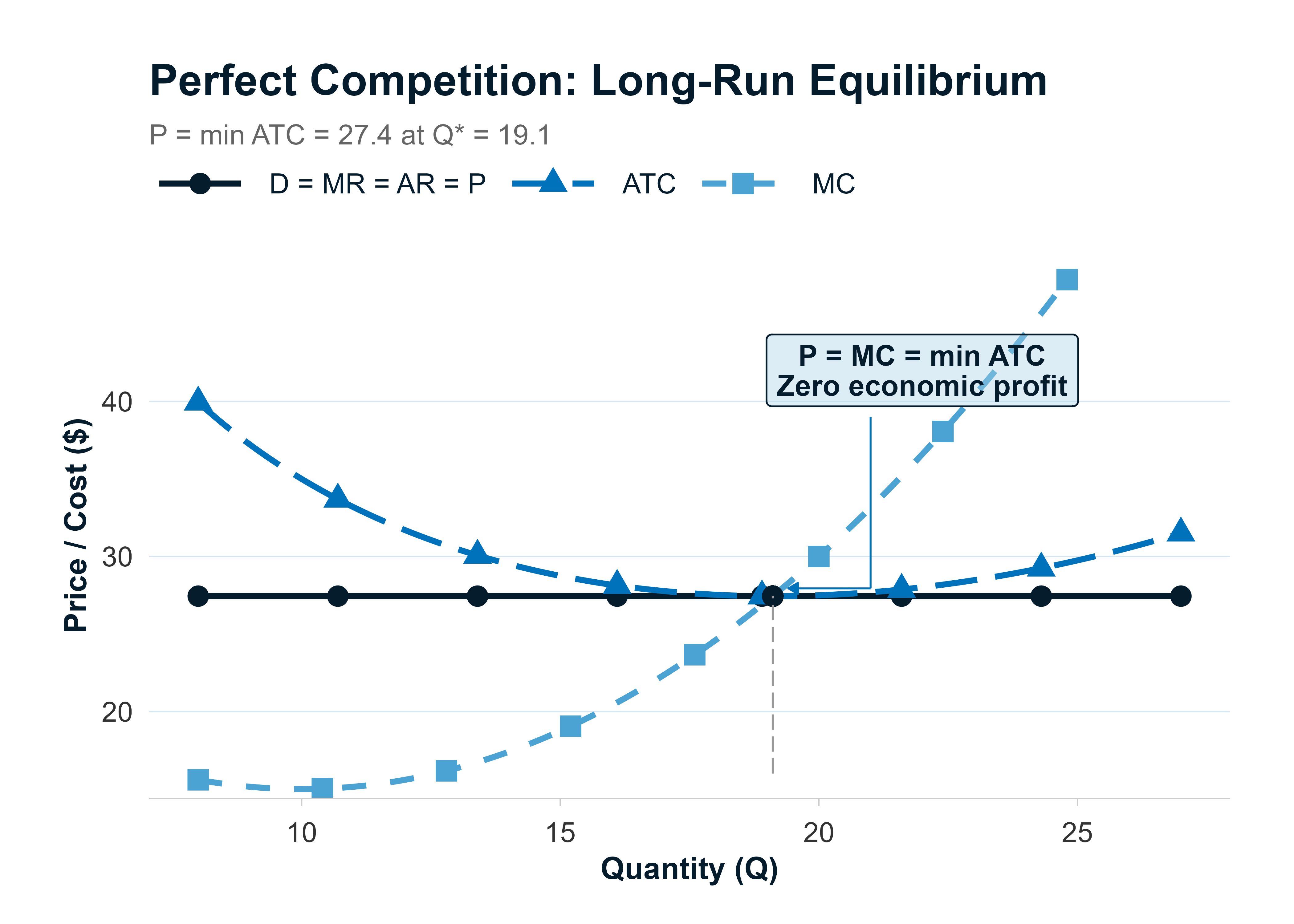
• In the long run, entry of new firms pushes economic profit to zero. Price settles at the minimum of average total cost.

Profit Maximization

The rule is the same for every market structure.

For a price-taker, marginal revenue equals the market price, so the rule simplifies to P = MC. The firm expands output until the cost of the last unit just equals the revenue it brings in.

---

Breakeven and Shutdown Analysis

Now that you know the benchmark of perfect competition, the next question is: when should a firm keep going, and when should it call it quits?

Cost Refresher

A quick reminder on cost terms:

• Fixed costs (FC): costs that do not change with output (rent, a signed lease, insurance). These exist only in the short run.
• Variable costs (VC): costs that rise and fall with output (raw materials, hourly wages).
• Total cost (TC) = FC + VC.
• Average total cost (ATC) = TC / Q.
• Average variable cost (AVC) = VC / Q.

In the short run, at least one factor of production (usually plant and equipment) is fixed. In the long run, all factors are variable. The firm can let leases expire and sell equipment, so every cost becomes avoidable.

The Three-Tier Decision Rule

There are only three scenarios. Memorize the table below and you can answer any shutdown question.

Condition	Short-Run Decision	Long-Run Decision
AR >= ATC (equivalently TR >= TC)	Operate; earning economic profit or breaking even	Stay in the market
AVC <= AR < ATC (equivalently TVC <= TR < TC)	Operate; losses are less than fixed costs	Exit the market
AR < AVC (equivalently TR < TVC)	Shut down; losses exceed fixed costs	Exit the market

Breakeven Point

The breakeven point is where economic profit equals zero.

Say a firm produces 10,000 units. ATC is $42 per unit. The market price is also $42.

Economic profit = $420,000 - $420,000 = $0. The firm is exactly at its breakeven point.

Short-Run Shutdown Point

Short-run shutdown: AR < AVC (equivalently, TR < TVC)

If revenue does not even cover variable costs, every unit the firm produces makes the loss worse. The firm is better off closing and just paying the fixed costs it owes anyway.

Imagine you signed a one-year lease on a food truck for $2,000 a month. Even if business is slow, you still owe the lease. The question is not "Am I making money?" but "Am I losing less by staying open than by closing?"

Worked Example: Short-Run Shutdown

A furniture maker reports total revenue of $520,000, total variable costs of $580,000, and total fixed costs of $300,000.

Total cost = $580,000 + $300,000 = $880,000.

Is TR >= TVC? $520,000 < $580,000. No.

The firm should shut down in the short run.

• Loss if operating = TC - TR = $880,000 - $520,000 = $360,000
• Loss if shut down = TFC = $300,000

Shutting down saves $60,000. The firm loses less by closing the doors.

Worked Example: Continue (Short Run), Exit (Long Run)

The same furniture maker now has a better quarter. Total revenue rises to $650,000 while costs stay the same (TVC = $580,000, TFC = $300,000).

Total cost = $580,000 + $300,000 = $880,000.

Is TR >= TVC? $650,000 >= $580,000. Yes. Is TR >= TC? $650,000 < $880,000. No.

The firm should continue operating in the short run.

• Loss if operating = $880,000 - $650,000 = $230,000
• Loss if shut down = $300,000

Operating saves $70,000 compared to shutting down, exactly the amount by which revenue exceeds variable cost ($650,000 - $580,000 = $70,000). In the long run, however, the firm should exit because TR < TC.

Shutdown Under Imperfect Competition

For a price-taker, comparing P to ATC and AVC works perfectly because price equals average revenue equals marginal revenue. Under imperfect competition (where the demand curve slopes downward), price no longer equals marginal revenue.

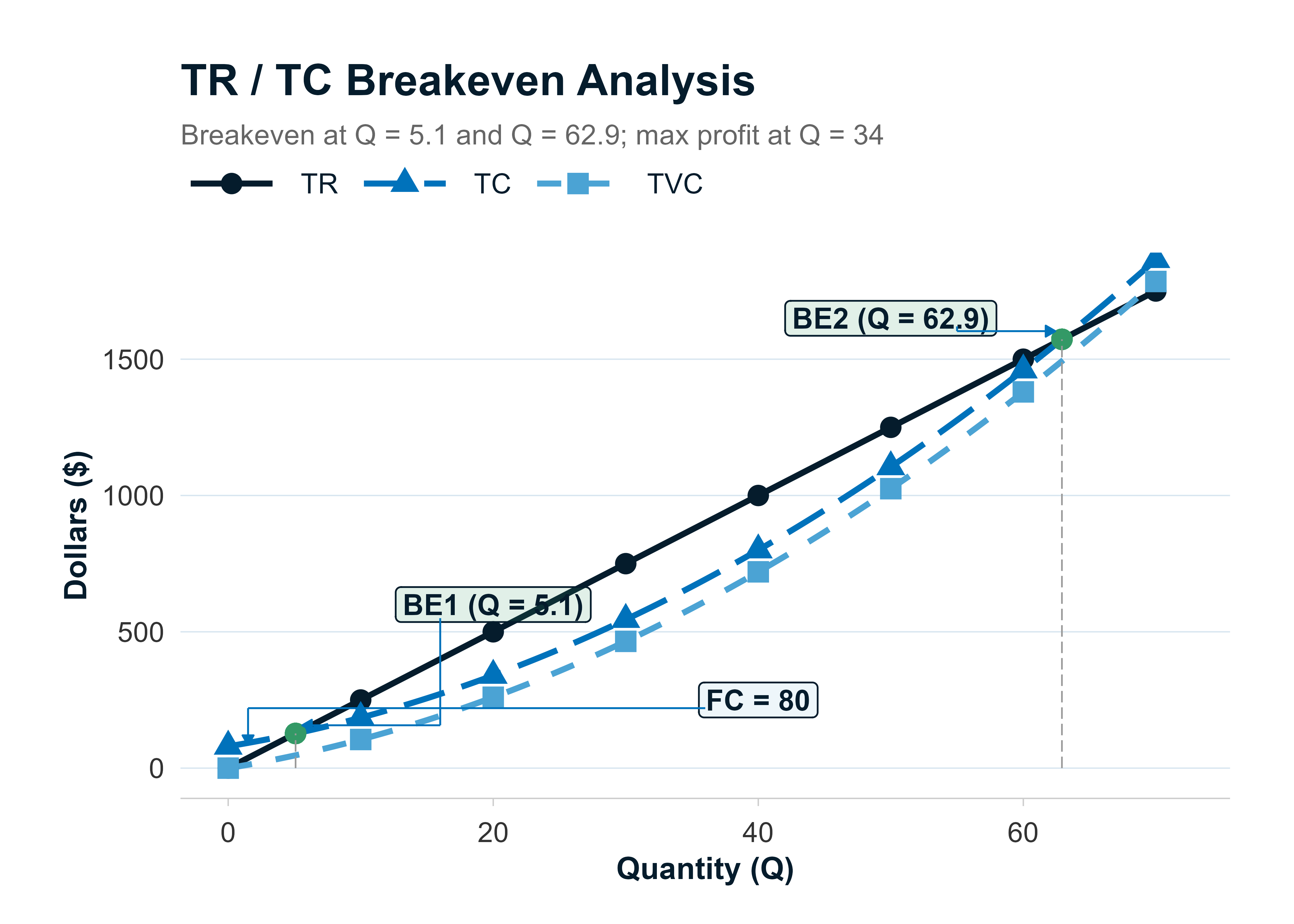
The safer approach is to use totals:

• TR = TC: breakeven
• TVC <= TR < TC: operate short run, exit long run
• TR < TVC: shut down immediately

The logic is identical. Only the labels change.

Exhibit 1

Trigger phrase in a question	What to do
"Should the firm shut down?"	Compare TR to TVC (short run) and TR to TC (long run)
"Firm has losses but..."	Check if TR >= TVC; if yes, keep operating short run
"Breakeven"	Set P = ATC or TR = TC
"Minimize losses in short run"	Continue if TR >= TVC
"Exit the market"	Long-run decision; exit if TR < TC

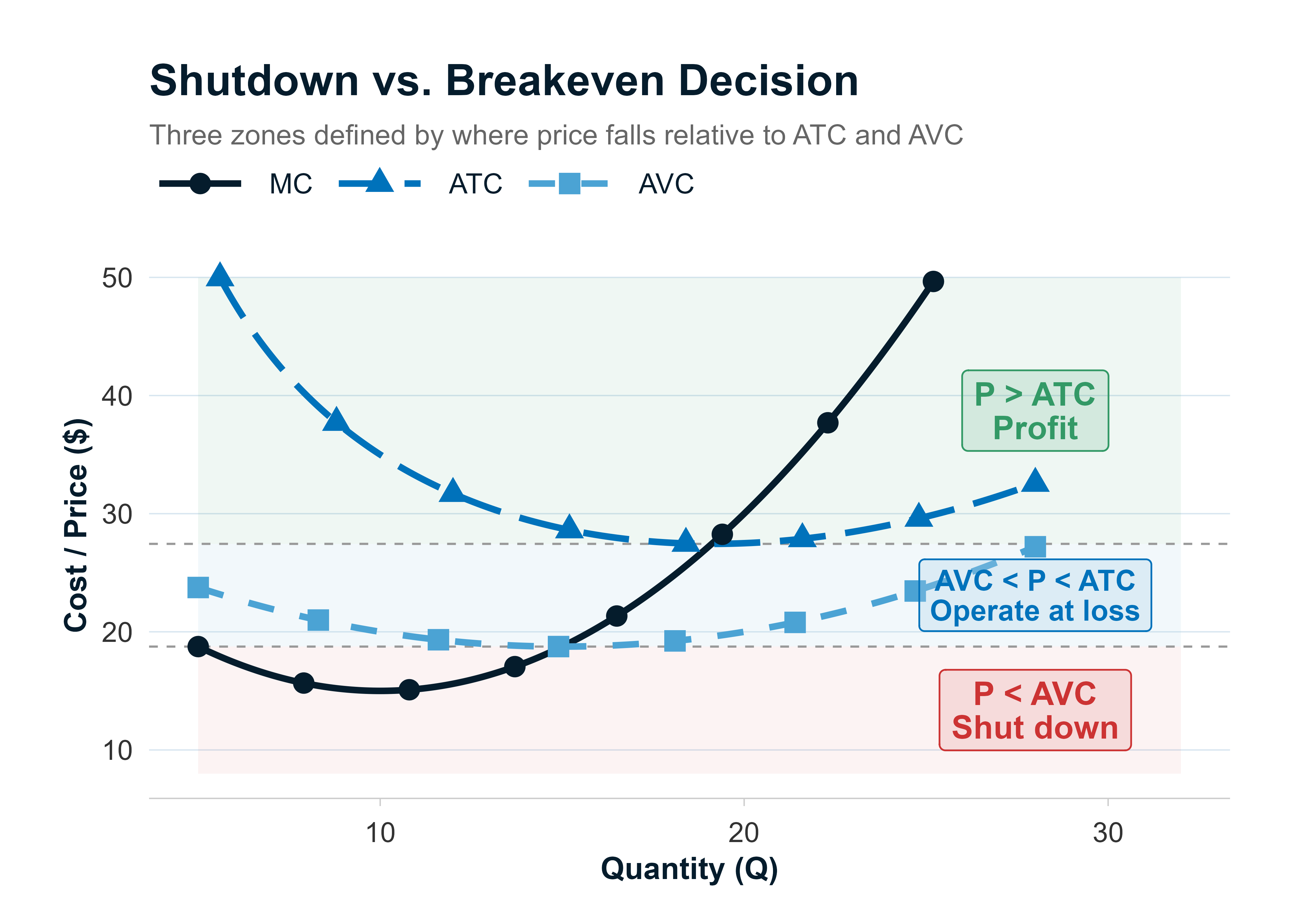
The diagram below shows the same logic on a per-unit cost curve chart. Three zones emerge, defined by where the market price sits relative to the cost curves:

• Price above ATC (green zone): the firm earns economic profit on every unit. This is the breakeven threshold - if P = min ATC, profit is exactly zero.
• Price between AVC and ATC (blue zone): the firm loses money overall, but revenue still covers all variable costs plus part of fixed costs. Operating is better than shutting down in the short run.
• Price below AVC (red zone): revenue does not even cover variable costs. Every unit produced increases the loss. The firm should shut down immediately.

Exhibit 2

---

Economies and Diseconomies of Scale

In the short run, plant size is fixed. But in the long run, a firm can build a bigger factory, add production lines, or downsize. The long-run average total cost (LRATC) curve shows the lowest possible ATC at each output level when the firm is free to adjust its scale.

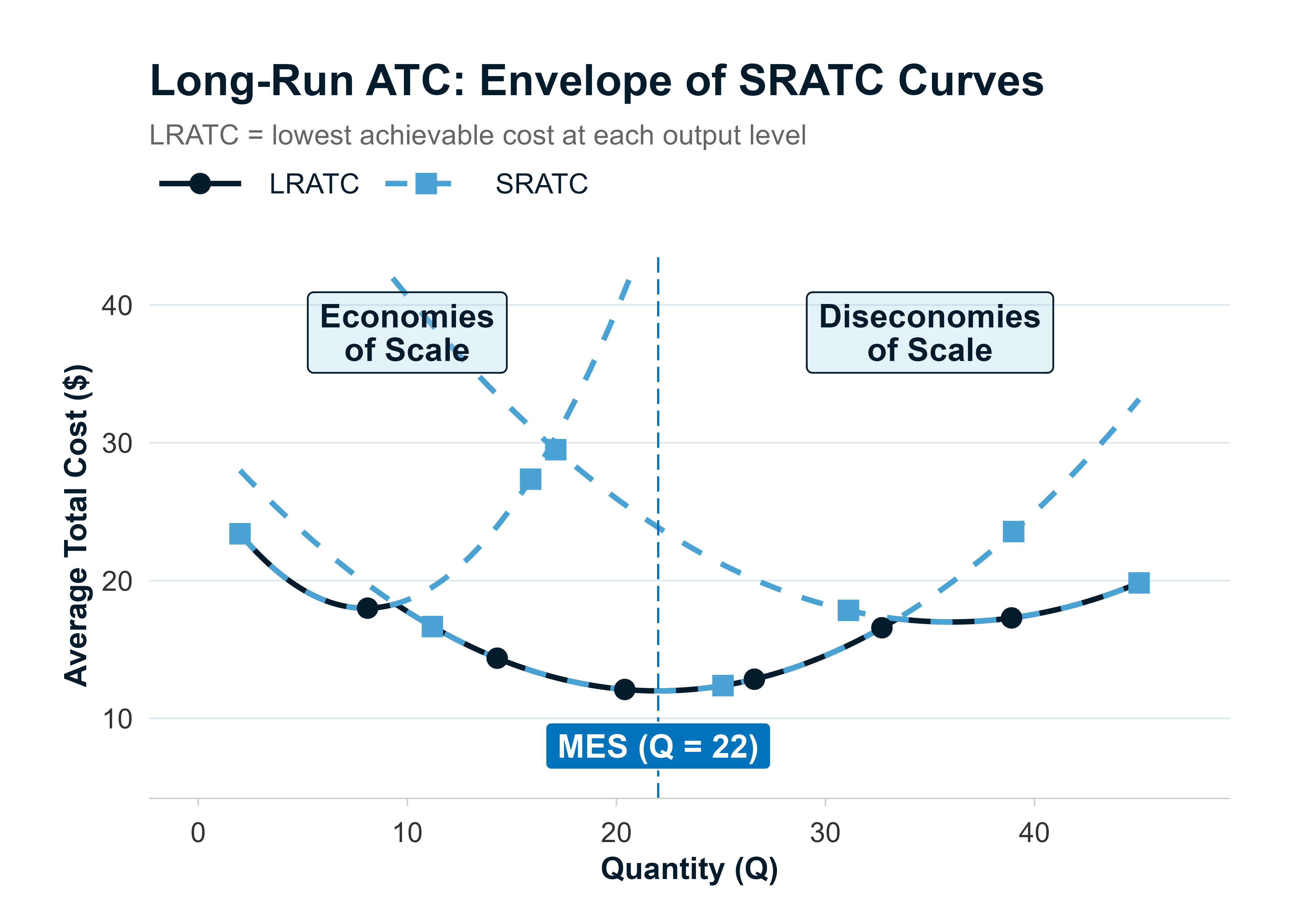
Picture the LRATC as a wide, shallow U-shape. It is drawn by tracing the bottom edge of many short-run ATC curves (one for each plant size). That is why it is often called an "envelope" curve.

Exhibit 3

Three Zones of the LRATC

Economies of scale (downward-sloping segment). As the firm grows, average cost falls. Bigger factories benefit from specialization, bulk purchasing, and more efficient equipment. A firm in this zone can cut costs by expanding.

Constant returns to scale (flat segment). Average cost stays roughly the same across a range of sizes. Growing does not help or hurt.

Diseconomies of scale (upward-sloping segment). The firm has gotten too big. Bureaucracy, communication problems, and difficulty motivating a large workforce push costs higher. A firm in this zone should consider scaling back.

Minimum Efficient Scale

The point where the LRATC first bottoms out is called the minimum efficient scale (MES). Under perfect competition, firms must operate at MES in long-run equilibrium. Any firm with higher average costs will suffer losses and eventually exit.

---

Monopolistic Competition

Monopolistic competition sits just one step away from perfect competition on the spectrum. There are still many firms and low barriers to entry, but each firm sells a slightly different product.

Think about the toothpaste aisle. Dozens of brands, all doing roughly the same thing. But each brand tries to stand out through whitening claims, flavor, packaging, or celebrity endorsements. Customers have favorites and will not switch the instant a rival drops its price by a penny. That is product differentiation in action.

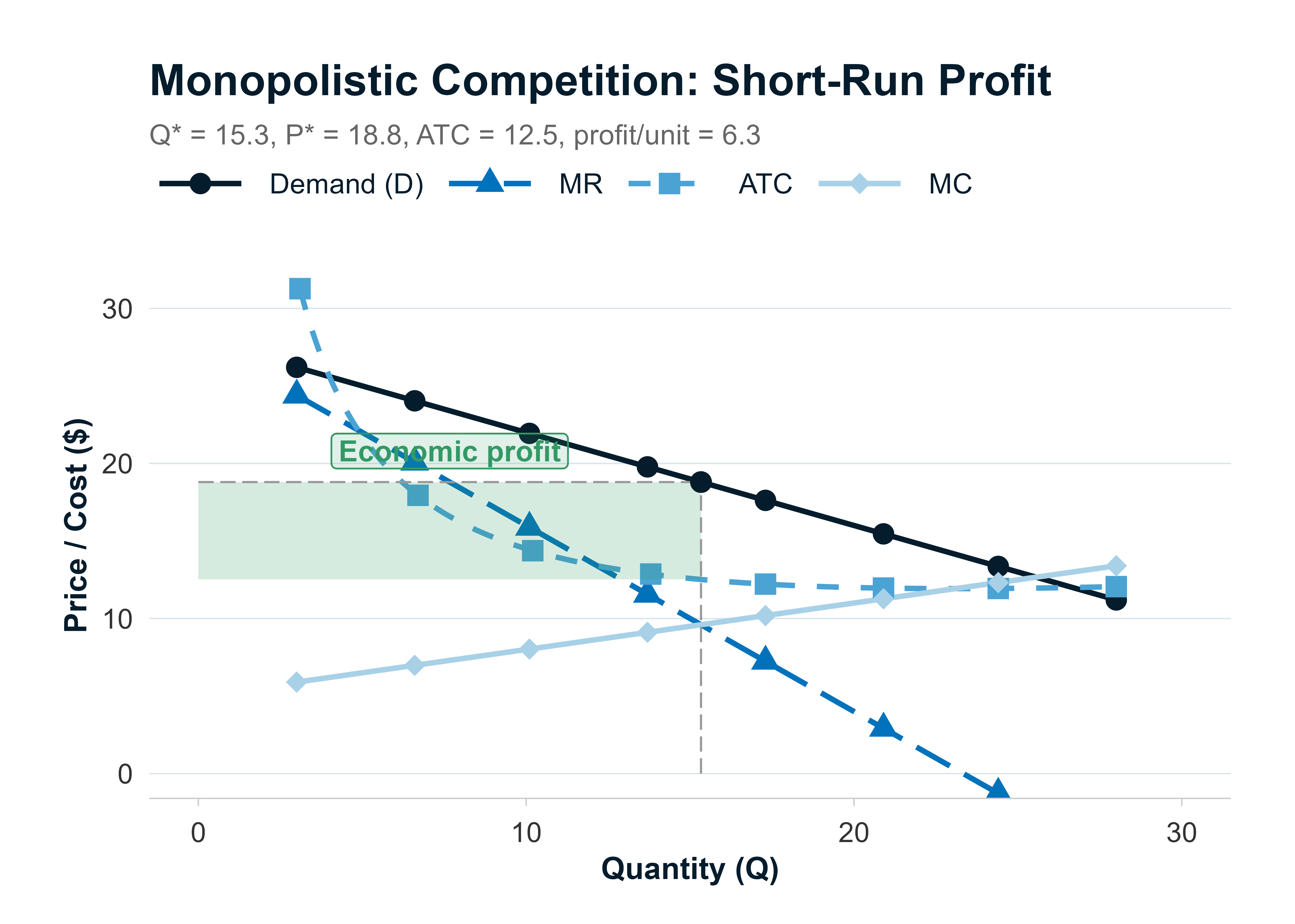
Short-Run Equilibrium

Because each firm's product is a little different, the firm faces a downward-sloping demand curve (not horizontal like a perfect competitor). Marginal revenue is less than price.

The firm still maximizes profit at MR = MC. In the short run, if the price at the profit-maximizing quantity exceeds ATC, the firm earns positive economic profit.

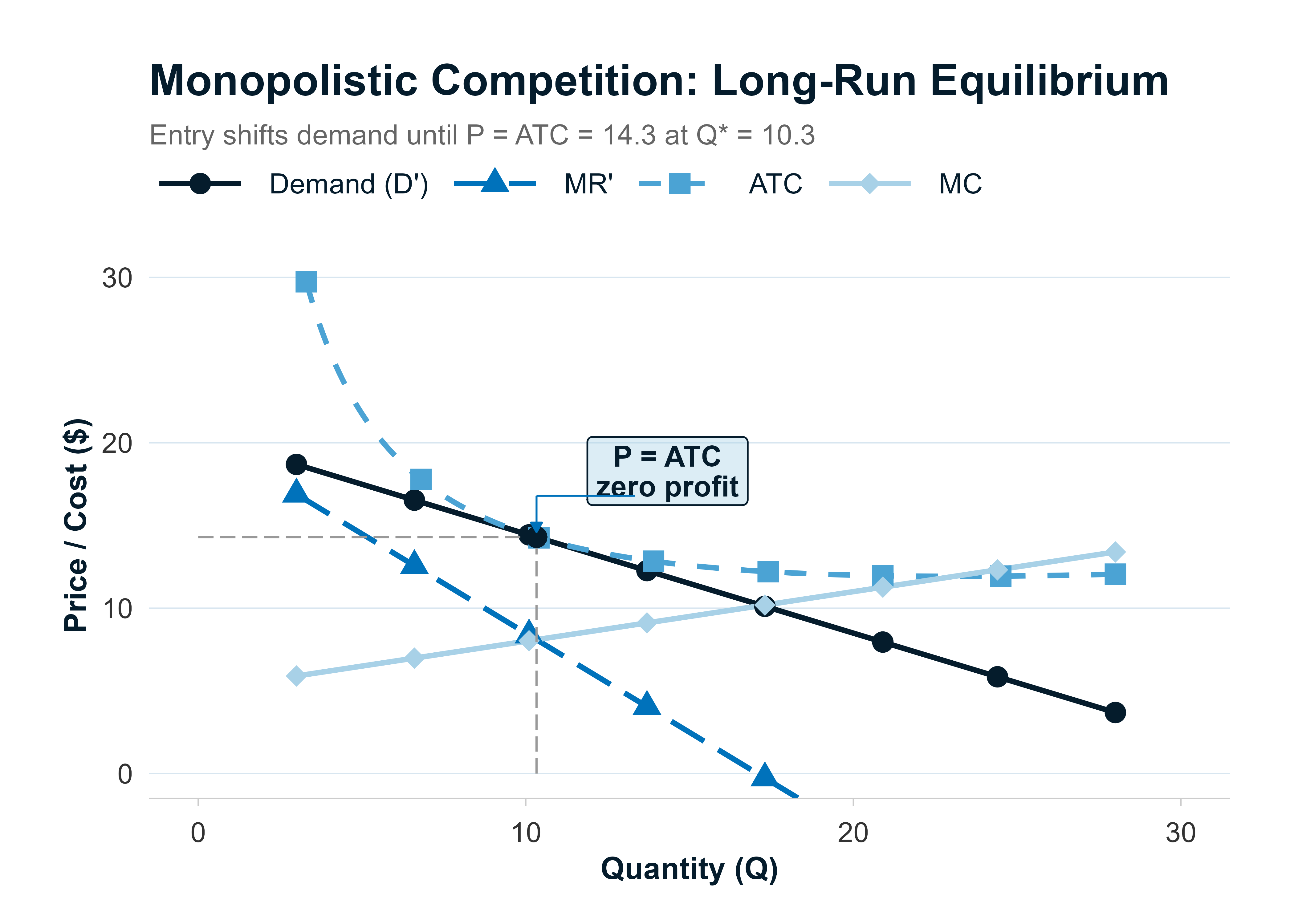
Long-Run Equilibrium

Positive profits attract new entrants. As new firms enter and offer close substitutes, each existing firm loses some customers. Its demand curve shifts down (leftward) until price equals ATC and economic profit drops to zero.

Two forces can eliminate short-run profits:

1. Entry of new competitors. Each firm's slice of the market shrinks.
2. Increased marketing spending. Firms ramp up advertising to protect their share. This pushes ATC up until it meets the price.

Either way, the long-run result is the same: P = ATC and zero economic profit.

Exhibit 4

Exhibit 5

Exhibit 6

Exhibit 7

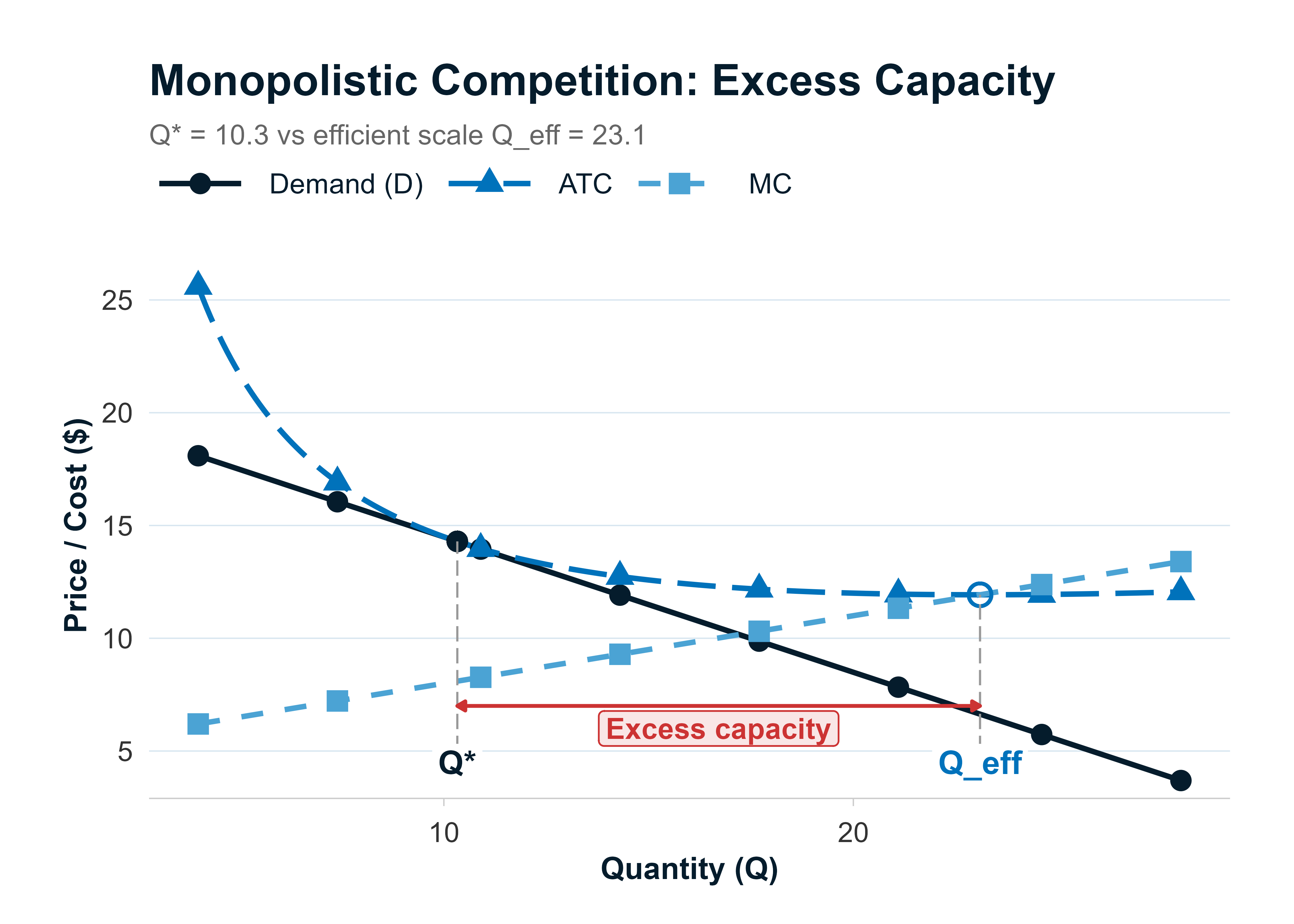
Excess Capacity

In long-run equilibrium, the firm does not produce at the minimum of its ATC curve. It produces at a point where ATC is still falling. This gap between the firm's output and the output at minimum ATC is called excess capacity.

The result: prices under monopolistic competition are slightly higher, and quantities slightly lower, than under perfect competition. Is that bad? Not necessarily. Consumers get variety. Whether the efficiency cost of that variety is "worth it" is the central trade-off.

---

Oligopoly

An oligopoly has just a few firms, high barriers to entry, and one defining feature: interdependence. Every firm must think about how rivals will react before making a pricing or output decision.

The automobile industry is a classic example. When one major manufacturer cuts prices, the others must respond or lose sales. That mutual awareness is what separates oligopoly from monopolistic competition, where each firm is too small to worry about any single rival.

Products in an oligopoly can be similar (crude oil) or differentiated (automobiles). Demand curves slope downward, and the degree of elasticity depends on how close the substitutes are.

Profit Maximization

The rule remains MR = MC. But in an oligopoly, figuring out the demand curve (and therefore MR) is the hard part, because it depends on what rivals do. Several models try to answer that question.

The Kinked Demand Curve Model

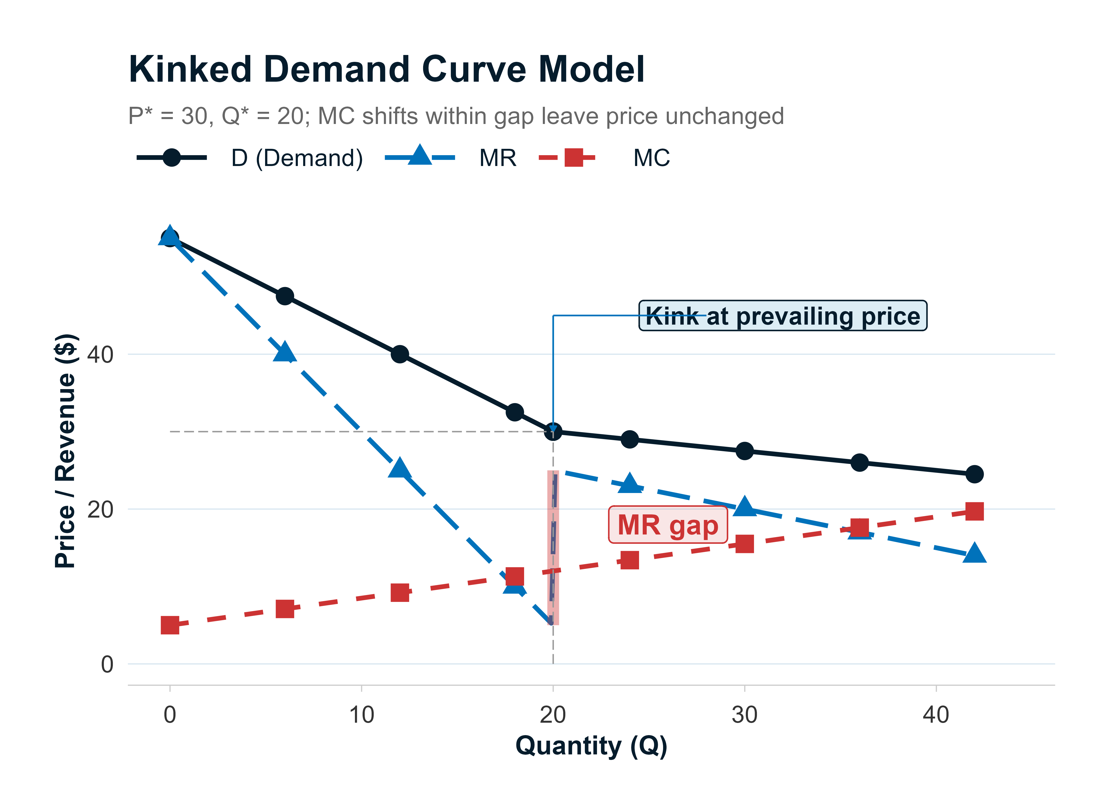
This model starts with one assumption: rivals will match your price cuts but will not match your price increases.

If you raise your price, customers leave quickly (rivals keep their lower price), so demand above the current price is very elastic. If you cut your price, rivals cut too, so you gain very few new customers; demand below the current price is relatively inelastic.

The result is a "kink" in the demand curve at the current price. Below the kink, the demand curve is steep. Above the kink, it is flat.

Because of the kink, there is a vertical gap in the MR curve. As long as the firm's MC curve passes through that gap, the firm has no incentive to change its price. This explains why oligopoly prices can be "sticky" even when costs shift moderately.

Exhibit 8

The Cournot Duopoly Model

The Cournot model assumes two firms with identical cost structures choose their prices simultaneously. Each firm picks its best price assuming the other firm's price stays the same.

In long-run equilibrium, both firms end up with equal market shares. The equilibrium price lands between the monopoly price (the highest) and the perfectly competitive price (the lowest). As more firms enter, the price moves closer to the competitive level.

The Stackelberg Dominant Firm Model

The Stackelberg model changes one thing: pricing decisions are sequential rather than simultaneous. One firm (the "leader") sets its price first. The other firm (the "follower") then responds.

The leader has a first-mover advantage. In long-run equilibrium, the leader captures a larger market share and earns more profit than the follower.

Nash Equilibrium

A Nash equilibrium is a set of strategies where no firm can increase its profits by changing its own strategy alone, given what every other firm is doing.

Think of two drivers arriving at an intersection at the same time. Each picks a strategy (go or wait). A Nash equilibrium is when neither driver wants to change their choice, given what the other driver is doing.

The Cournot equilibrium is a Nash equilibrium. Neither firm can do better by unilaterally changing its price.

Worked Example: Nash Equilibrium from a Payoff Matrix

Two coffee shops, Brew Co. and Grind Inc., each choose between a High Price and a Low Price strategy. Their weekly profits (in dollars) are shown below.

	Grind: High Price	Grind: Low Price
Brew: High Price	Brew = 800, Grind = 500	Brew = 300, Grind = 650
Brew: Low Price	Brew = 900, Grind = 350	Brew = 450, Grind = 400

Brew Co.'s analysis:

• If Grind chooses High: Brew gets 800 (High) or 900 (Low). Brew prefers Low.
• If Grind chooses Low: Brew gets 300 (High) or 450 (Low). Brew prefers Low.
• Brew has a dominant strategy: Low Price.

Grind Inc.'s analysis:

• If Brew chooses High: Grind gets 500 (High) or 650 (Low). Grind prefers Low.
• If Brew chooses Low: Grind gets 350 (High) or 400 (Low). Grind prefers Low.
• Grind has a dominant strategy: Low Price.

Nash equilibrium: both choose Low Price. Brew earns 450 and Grind earns 400. Neither firm can improve its profit by switching to High while the other stays at Low.

Notice the irony: if both chose High, joint profits would be 800 + 500 = 1,300 instead of 450 + 400 = 850. But neither firm trusts the other to keep prices high, so both end up worse off. This is the classic incentive problem behind collusion.

Collusion and Cartels

Collusion occurs when competing firms agree to set prices or restrict output jointly. If they succeed, the group behaves like a monopoly, charging the monopoly price and splitting the monopoly profit.

A cartel is a formal collusion arrangement. The most famous example is a group of oil-producing nations that agrees to cap production and drive up world oil prices.

Collusion is more likely to hold together when:

• There are fewer firms (easier to coordinate).
• Products are more similar (less temptation to compete on features).
• Cost structures are more similar (equal incentive to cooperate).
• Purchases are small and frequent (cheating is detected quickly).
• Retaliation is severe and certain (high cost of breaking the deal).
• There is less outside competition (no one to undercut the group).

Collusion is illegal in many countries because it harms consumers by raising prices above the competitive level.

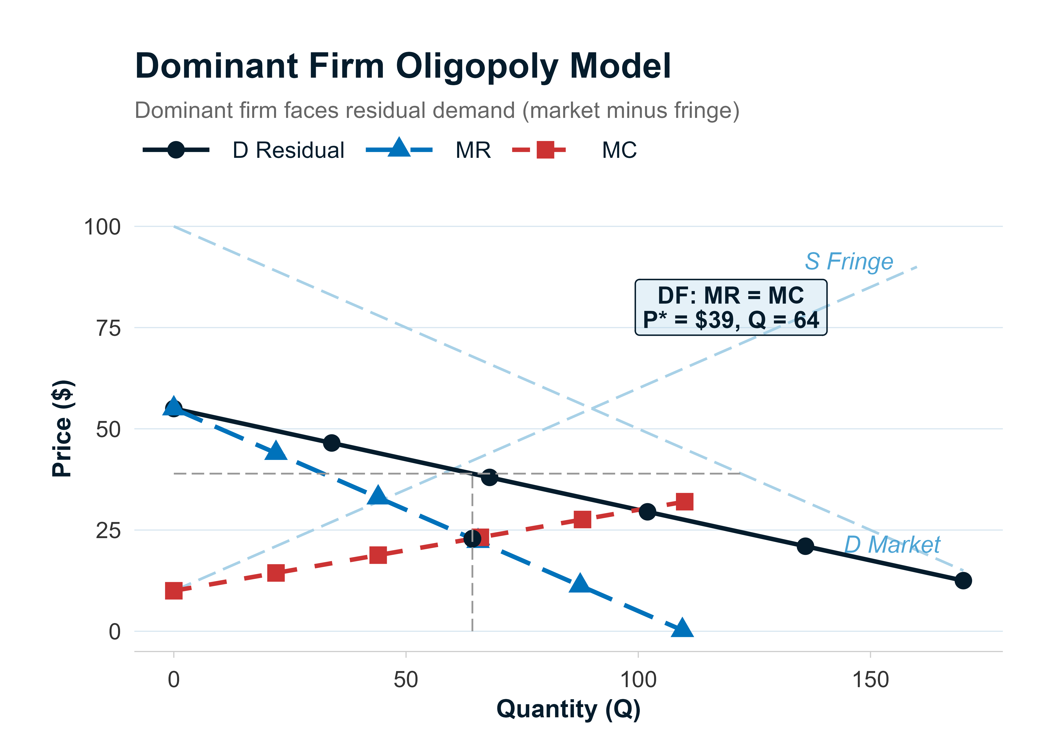
The Dominant Firm Model

Sometimes one firm has a much larger market share and lower costs than everyone else. That firm is the dominant firm (DF). The remaining small firms are the competitive fringe (CF).

The DF effectively sets the market price. The CF firms are price-takers; they produce whatever quantity makes their marginal cost equal to the price the DF sets.

If a fringe firm tries to undercut the DF's price, the DF can respond by cutting its own price further (it has the cost advantage). In the long run, the fringe firm either exits or shrinks, and the DF's market share grows.

Exhibit 9

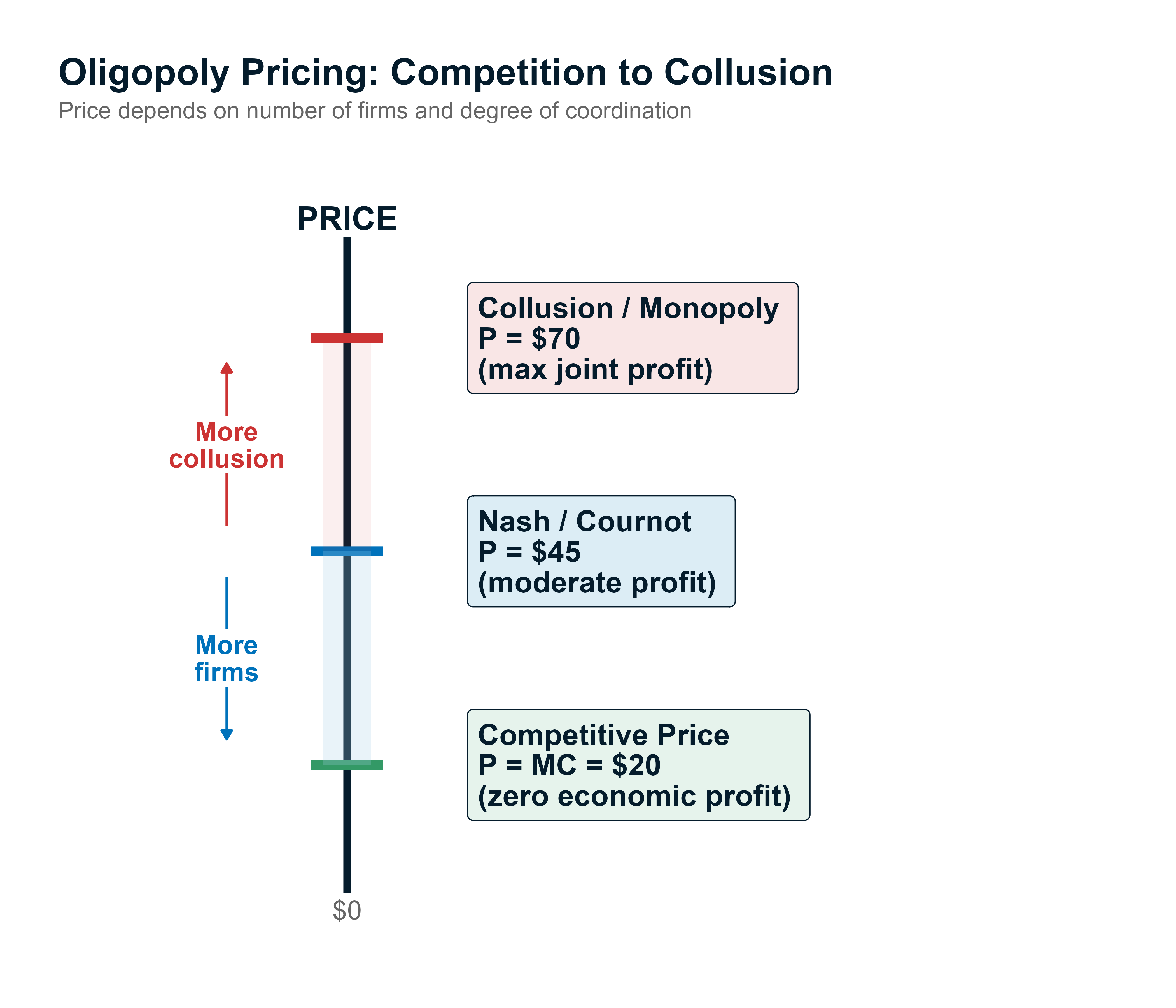
Oligopoly Price Range

The most important takeaway on oligopoly pricing is that the actual market price falls somewhere between two extremes:

• Upper bound: the collusion (monopoly) price, where all firms coordinate to maximize joint profit.
• Lower bound: the perfectly competitive price, where economic profit is zero.

Where exactly the price lands depends on how many firms exist, how interdependent they are, and which pricing model best describes their behavior.

Exhibit 10

Oligopoly Model	Key Assumption	LR Market Share
Kinked demand	Rivals match cuts, ignore increases	Stable at current levels
Cournot	Simultaneous pricing, identical costs	Equal shares
Stackelberg	Sequential pricing (leader then follower)	Leader gets more
Nash equilibrium	No firm gains from unilateral change	Varies by game
Dominant firm	One firm has lowest costs	DF gets largest share

---

Pure Monopoly

A monopoly is the far end of the spectrum: a single firm with no close substitutes and very high barriers to entry.

Monopoly power can come from patents, control of a critical resource, or government regulation (a local electric utility, for instance). The monopolist faces the entire market demand curve, which slopes downward.

Because the monopolist is the market, it has significant pricing power. It still maximizes profit where MR = MC, but it can set the price above marginal cost and earn positive economic profit even in the long run, as long as barriers prevent entry.

---

Identifying Market Structures

In practice, you rarely see a textbook-perfect example of any structure. Markets are messy. But you can get a useful estimate of how competitive a market is by looking at concentration measures.

N-Firm Concentration Ratio

The simplest measure. Add up the market shares (as percentages) of the N largest firms.

where:

• s_i = percentage market share of the i-th largest firm

Herfindahl-Hirschman Index (HHI)

A more refined measure. Square each firm's market share (expressed as a decimal), then add them up.

where:

• s_i = market share of the i-th largest firm, expressed as a decimal (not a percentage)

Worked Example: Concentration Ratio and HHI

Five firms have the following market shares: Firm A = 30%, Firm B = 25%, Firm C = 20%, Firm D = 15%, Firm E = 10%.

4-firm concentration ratio:

4-firm HHI:

Worked Example: Merger Impact

Now suppose Firms A and B merge. The new combined firm has 55% of the market (30% + 25%).

Post-merger shares: AB = 55%, C = 20%, D = 15%, E = 10%.

4-firm concentration ratio (post-merger):

4-firm HHI (post-merger):

The concentration ratio rose from 90% to 100% (up 10 percentage points). The HHI jumped from 0.2150 to 0.3750 (up 0.1600). That is a 74.4% jump in HHI versus an 11.1% jump in the concentration ratio. The HHI captures the merger's impact far more dramatically.

Why HHI Is More Sensitive

Because the HHI squares each share, large firms contribute disproportionately. When two big firms merge, the squared term of the combined entity is much larger than the sum of the two original squared terms. The simple concentration ratio just adds percentages, so it barely moves when two top firms combine.

Limitations of Both Measures

Neither the concentration ratio nor the HHI is perfect:

• Neither accounts for barriers to entry. A firm may have a large market share but little pricing power if new competitors can enter easily.
• Neither measures demand elasticity directly. High concentration does not guarantee high prices; potential competition can keep firms honest.
• The concentration ratio is relatively insensitive to mergers among top firms. It can stay the same even when two large firms combine, because the sum of their shares does not change.

Measure	Advantage	Key Limitation
N-firm ratio	Simple to calculate	Insensitive to mergers among top firms
HHI	More sensitive to mergers	Does not account for barriers to entry

---

Checklist

---

Practice Questions

1. A firm reports TR = $180,000, TVC = $200,000, and TFC = $120,000. What should the firm do in the short run?

A. Continue operating to cover part of its fixed costs B. Shut down because TR < TVC C. Continue operating because TR > TFC

2. A firm's price is $25, ATC is $25, and AVC is $18. Which condition best describes this firm?

A. The firm should shut down B. The firm is at its breakeven point C. The firm is earning positive economic profit

3. A firm expands its plant by 20% and its minimum ATC drops from $50 to $44. This firm is most likely experiencing:

A. Diseconomies of scale B. Constant returns to scale C. Economies of scale

4. A market has many firms, low barriers to entry, differentiated products, and some pricing power. This market is best characterized as:

A. Perfect competition B. Monopolistic competition C. Oligopoly

5. A firm in monopolistic competition has MC = $12 and MR = $12 at Q = 500. The price at Q = 500 is $18. The profit-maximizing output is:

A. Greater than 500 because P > MC B. Exactly 500 because MR = MC C. Less than 500 because P > MR

6. A firm in an oligopoly believes that its rivals will match price decreases but will not match price increases. This belief is most consistent with the:

A. Cournot model B. Stackelberg model C. Kinked demand model

7. Consider the following payoff matrix for Firm A and Firm B (profits in dollars):

	B: High Price	B: Low Price
A: High Price	A = 600, B = 400	A = 200, B = 500
A: Low Price	A = 700, B = 300	A = 350, B = 350

The Nash equilibrium is:

A. Both firms choose High Price B. A chooses High, B chooses Low C. Both firms choose Low Price

8. Seven firms have market shares of 35%, 20%, 15%, 10%, 8%, 7%, and 5%. The 3-firm concentration ratio is closest to:

A. 55% B. 70% C. 80%

9. Four firms have market shares of 40%, 25%, 20%, and 15%. The HHI for this market is closest to:

A. 0.1000 B. 0.2850 C. 0.3750

10. Using the market from Q9, the firms with 25% and 20% shares merge. The post-merger HHI is closest to:

A. 0.2850 B. 0.3000 C. 0.3850

11. A firm in monopolistic competition earns positive economic profit in the short run. In the long run, this firm's economic profit will most likely:

A. Remain positive because of product differentiation B. Become zero because low barriers allow new entry C. Become negative because advertising costs rise

12. Two firms in a duopoly have identical cost structures. Under which model will they share the market equally in long-run equilibrium?

A. Stackelberg B. Cournot C. Dominant firm